Surface Morphometrics Pipeline

Quantification of Membrane Surfaces Segmented from Cryo-ET or other volumetric imaging.

Author: Benjamin Barad/benjamin.barad@gmail.com.

Developed in close collaboration with Michaela Medina

A pipeline of tools to generate robust open mesh surfaces from voxel segmentations of biological membranes using the Screened Poisson algorithm, calculate morphological features including curvature and membrane-membrane distance using pycurv's vector voting framework, and tools to convert these morphological quantities into morphometric insights.

📖 Complete Quantifications Documentation - Reference guide for all morphological measurements and their interpretations.

Installation Options:

Option 1: Native Installation through Conda

This is the fastest and easiest starting point for most linux boxes, and now for mac as well

1. Clone this git repository: git clone https://github.com/grotjahnlab/surface_morphometrics.git
2. Install the conda environment: conda env create -f environment.yml
3. Activate the conda environment: conda activate morphometrics

Note: Older ubuntu installs (and probably some other linux distributions!) have some known issues with graph-tool. If you run into issues with the main environment file, try using environment-ubuntu.yml instead. This worked on my Ubuntu 22.04 LTS box.

Option 2: Docker Container

This allows operation on windows and other operating systems where graph-tool or pymeshlab do not play nice with each other or with conda.

1. Clone this git repository:

git clone https://github.com/grotjahnlab/surface_morphometrics.git
cd surface_morphometrics

2. Start the containerized environment:

cd docker
./sm-up.sh

This will pull and start the Docker container with all dependencies pre-installed. 3. When finished, exit the container and stop it:

exit # Exit the container
./sm-down.sh # Stop the container

Working with Docker Container

1. Starting a Session:

cd surface_morphometrics # Go to project directory
cd docker                # Enter docker directory
./sm-up.sh               # Start and enter container

2. Inside Container:

• The environment is pre-configured
• All dependencies are installed
• You can directly run the pipeline commands

3. Ending a Session:

exit           # Exit the container
./sm-down.sh   # Stop the container

Example data

There is tutorial segmentation data available in the example_data folder. Uncompress the tar file with:

cd example_data
tar -xzvf examples.tar.gz

There are two example datasets: TE1.mrc and TF1.mrc. No tomogram data is provided for refinement or thickness measurement, as these require larger files, but the segmentation files are sufficient to run the curvature and distance/orientation steps of the pipeline. You can open them with mrcfile, like so:

import mrcfile

with mrcfile.open('TE1.mrc', permissive=True) as mrc:
    print(mrc.data.shape)  # TE1.mrc has shape (312, 928, 960)

In some cases the file header may be non-standard (for example, mrc files exported from Amira software). In these cases, the permissive=True keyword argument is required, and you can ignore the warning that the file may be corrupt. All the surface morphometrics toolkit scripts will still run correctly.

Running the configurable pipeline

Running the full pipeline on a 4 core laptop with the tutorial datasets takes about 8 hours (3 for TE1, 5 for TF1), mostly in steps 3 and 4. With cluster parallelization, the full pipeline can run in 2 hours for as many tomograms as desired.

1. Edit the config.yml file for your specific project needs. New users: we recommend starting with isotropic_remesh: true and simplify: false in the surface_generation section for higher quality meshes with near-equilateral triangles. A target_area between 1.0 and 3.0 nm^2 generally yields good results, but smaller triangles significantly increase computation time. The default config uses simplify: true for faster processing.

   Note for existing users: two config keys were renamed for clarity. data_dir is now seg_dir (the directory of segmentation MRC files), and max_triangles is now simplify_max_triangles (only used when simplify: true). Update older config files accordingly — segmentation_to_meshes.py will print a warning if it detects the old names.

2. Run the surface reconstruction for all segmentations: python segmentation_to_meshes.py config.yml

3. Run pycurv for each surface (recommended to run individually in parallel with a cluster): python run_pycurv.py config.yml ${i}.surface.vtp

   You may see warnings aobut the curvature, this is normal and you do not need to worry.

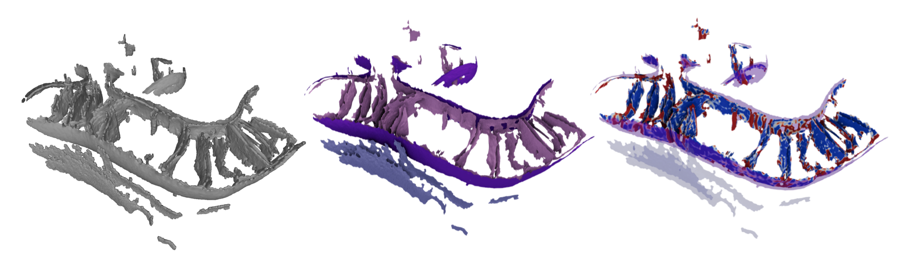
4. (Optional) Density-guided mesh refinement. After pycurv, and before the distance/orientation and thickness steps, you can refine the surface meshes so that vertices sit more accurately on the membrane bilayer center: python refine_mesh.py config.yml. This step samples the raw tomogram density along surface normals and iteratively recenters vertices on the fitted bilayer (or, in high-defocus data, a single Gaussian), re-running pycurv on each iteration. It requires raw tomograms in tomo_dir organized as described in Data organization for thickness and refinement below, since it reuses the same tomogram-to-surface matching as the thickness workflow. Refinement is most useful when segmentations are slightly offset from the true membrane center, and it improves the accuracy of all downstream measurements (curvature, distances, and thickness). Tuning options live in the mesh_refinement section of config.yml. Refinement writes a numbered surface per iteration (*_refined_iter*.surface.vtp and their AVV graphs) plus convergence plots, but does not automatically replace your working surfaces — you choose which iteration to keep with accept_refinement.py (below).

   Accepting a refinement iteration. Inspect the summaries (*_refinement_convergence.png, *_profile_evolution.png) to choose the best iteration, then commit it with python accept_refinement.py config.yml ${step} (where ${step} is the iteration number). This:

   • backs up the original surfaces to *.orig.bak (so the pre-refinement state is recoverable),

   • promotes the chosen iteration to be the main surface used by the remaining steps (keeping only the canonical *.surface.vtp and *.AVV_rh*.gt/.vtp/.csv),

   • and removes the other iterations, per-iteration plots, and regenerable pycurv intermediates, while keeping the refinement summaries.

     Useful options: --dry-run previews every rename/delete without touching files; --component_name OMM (or --tomogram TF1) restricts the operation to a subset of surfaces. By default it accepts the chosen iteration for every refined surface in work_dir.

     Note: intermediate cross-correlation iterations (when use_xcorr is enabled) are saved with a fast "lightweight" graph rather than a full pycurv curvature graph — only the final iteration always gets full pycurv. If you accept one of these lightweight iterations, the promoted surface will have no *.AVV_rh*.gt graph and is not ready for downstream analysis; accept_refinement.py will warn you and print the exact run_pycurv.py command to run on the accepted surface first.

5. Measure intra- and inter-surface distances and orientations (also best to run this one in parallel for each original segmentation): python measure_distances_orientations.py config.yml ${i}.mrc

6. For thickness (requires a tomo folder), first sample the density: python sample_density.py config.yml

7. For thickness, then run: python measure_thickness.py config.yml

8. Combine the results of the analysis into aggregate Experiments and generate statistics and plots. This requires some manual coding using the Experiment class and its associated methods in the morphometrics_stats.py. Everything is roughly organized around working with the CSVs in pandas dataframes. Running morphometrics_stats.py as a script with the config file and a filename will output a pickle file with an assembled "experiment" object for all the tomos in the data folder. Reusing a pickle file will make your life way easier if you have dozens of tomograms to work with, but it doesn't save too much time with just the example data...

Data organization for thickness and refinement

The thickness measurement (steps 6-7) and the optional mesh refinement (step 4) both read the raw tomogram density, not just the segmentation. Three directories in config.yml control this:

• seg_dir — the segmentation MRC files (the label volumes you generate surfaces from).
• tomo_dir — the raw (greyscale) tomogram MRC files that the segmentations were drawn on.
• work_dir — the working/output directory where pycurv writes its graphs (.gt) and CSVs.

The critical requirement is that each raw tomogram in tomo_dir must share the same basename (the part of the filename before .mrc) as its segmentation. Tomograms are matched to surfaces by globbing work_dir for files named like {tomogram_basename}*{component}.AVV_rh{radius_hit}.gt. For example, if your segmentation is TE1.mrc (producing graphs such as TE1_OMM.AVV_rh9.gt), the raw tomogram must also be named TE1.mrc and placed in tomo_dir. A typical layout:

project/
├── segmentations/   # seg_dir  →  TE1.mrc, TF1.mrc   (label volumes)
├── tomograms/       # tomo_dir  →  TE1.mrc, TF1.mrc   (raw density, matching basenames)
└── morphometrics/   # work_dir  →  TE1_OMM.AVV_rh9.gt, ... (pycurv output + results)

Sampling output (*_sampling.csv) is written into work_dir alongside the graph files. If no graph files matching a tomogram's basename are found, that tomogram is silently skipped — so a basename mismatch is the most common reason thickness or refinement "finds no files."

Examples of generating statistics and plots:

• python single_file_histogram.py filename.csv -n feature will generate an area-weighted histogram for a feature of interest in a single tomogram. I am using a variant of this script to respond to reviews asking for more per-tomogram visualizations!
• python single_file_2d.py filename.csv -n1 feature1 -n2 feature2 will generate a 2D histogram for 2 features of interest for a single surface.
• mitochondria_statistics.py shows analysis and comparison of multiple experiment objects for different sets of tomograms (grouped by treatment in this case). Every single plot and statistic in the preprint version of the paper gets generated by this script.

Running individual steps without pipelining

Individual steps are available as click commands in the terminal, and as functions

1. Robust Mesh Generation
   1. mrc2xyz.py to prepare point clouds from voxel segmentation
   2. xyz2ply.py to perform screened poisson reconstruction and mask the surface
   3. ply2vtp.py to convert ply files to vtp files ready for pycurv
2. Surface Morphology Extraction
   1. curvature.py to run pycurv in an organized way on pregenerated surfaces
   2. (Optional) refine_mesh.py to density-guide the surface onto the membrane bilayer center after pycurv, before the distance and thickness steps. Requires raw tomograms (see Data organization for thickness and refinement). Then accept_refinement.py config.yml ${step} to commit a chosen iteration as the new working surface (backs up the originals to *.orig.bak and cleans up the intermediates; use --dry-run to preview).
   3. intradistance_verticality.py to generate distance metrics and verticality measurements within a surface.
   4. interdistance_orientation.py to generate distance metrics and orientation measurements between surfaces.
   5. sample_density.py then measure_thickness.py to measure local membrane thickness from the raw tomogram density.
   6. Outputs: gt graphs for further analysis, vtp files for paraview visualization, and CSV files for pandas-based plotting and statistics
3. Morphometric Quantification - there is no click function for this, as the questions answered depend on the biological system of interest!
   1. morphometrics_stats.py is a set of classes and functions to generate graphs and statistics with pandas.
   2. Paraview for 3D surface mapping of quantifications.
   3. Quantifications Documentation - Complete reference for all morphological measurements and their interpretations.

File Descriptions:

• Files with.xyz extension are point clouds converted, in nm or angstrom scale. This is a flat text file with X Y Z coordinates in each line.
• Files with .ply extension are the surface meshes (in a binary format), which will be scaled in nm or angstrom scale, and work in many different softwares, including Meshlab.
• Files with .vtp extension are the same surface meshes in the VTK format. * The .surface.vtp files are a less cross-compatible format, so you can't use them with as many types of software, but they are able to store all the fun quantifications you'll do!. Paraview or pyvista can load this format. This is the format pycurv reads to build graphs. * The .AVV_rh8.vtp files are those output from downstream components of the pipeline, and generally have the most available visualizations in paraview and pyvista.
• Files with .gt extension are triangle graph files using the graph-tool python toolkit. These graphs enable rapid neighbor-wise operations such as tensor voting, but are not especially useful for manual inspection.
• Files with .csv extension are quantification outputs per-triangle. These are the files you'll use to generate statistics and plots.
• Files with .log extension are log files, mostly from the output of the pycurv run.
• Quantifications (plots and statistical tests) are output in csv, svg, and png formats.

Troubleshooting

1. Warnings of the type Gaussian or Mean curvature of X has a large computation error... can be ignored, as they get cleaned up by pycurv. These warnings are now suppressed by default.
2. MRC files that are output by AMIRA don't have proper machine stamps by default. They need to be imported with mrcfile.open(filename, permissive=True). This is also true for many other softwares, including Dragonfly.
3. Pycurv has recently undergone significant performance improvements and has more feedback; if it seems to be hanging indefinitely, try setting cores to 1 in the config file.

Dependencies

1. Numpy
2. Scipy
3. Pandas
4. mrcfile
5. Click
6. Matplotlib
7. Pymeshlab
8. Pycurv
   1. Pyto
   2. Graph-tool

Citation

The development of this toolkit and examples of useful applications can be found in the following manuscript. Please cite it if you use this software in your research, or extend it to make improvements!

Quantifying organellar ultrastructure in cryo-electron tomography using a surface morphometrics pipeline. Benjamin A. Barad^†, Michaela Medina^†, Daniel Fuentes, R. Luke Wiseman, Danielle A. Grotjahn Journal of Cell Biology 2023, 222(4), e202204093; doi: https://doi.org/10.1083/jcb.202204093

Thickness measurement is described in this manuscript:

Surface Morphometrics reveals local membrane thickness variation in organellar subcompartments. Michaela Medina^†, Ya-Ting Chang^†, Hamidreza Rahmani, Mark Frank, Zidan Khan, Daniel Fuentes, Frederick A. Heberle, M. Neal Waxham, Benjamin A. Barad^✉, Danielle A. Grotjahn^✉. Journal of Cell Biology 2025, 225(3), e202505059, doi: https://doi.org/10.1083/jcb.202505059

All scientific software is dependent on other libraries, but the surface morphometrics toolkit is particularly dependent on PyCurv, which provides the vector voted curvature measurements and the triangle graph framework. As such, please also cite the pycurv manuscript:

Reliable estimation of membrane curvature for cryo-electron tomography.
Maria Salfer,Javier F. Collado,Wolfgang Baumeister,Rubén Fernández-Busnadiego,Antonio Martínez-Sánchez
PLOS Comp Biol August 2020; doi: https://doi.org/10.1371/journal.pcbi.1007962